6  Annotation and Downstream Analysis

Now that we have our sets of differentially expressed genes, we can now do the following:

• Cluster and visualize the clusters in a heatmap
• Annotate our gene sets on annotations, pathways, or networks

graph TD
A[Differential Analysis] --> B[Gene Set Analysis]
A --> C[Clustering and Visualization]

6.1 What Now?

There are various approches we can do with our DE gene set. If it is large, we may want to try to filter and then cluster the genes to find groups of similar function. The assumption here is that genes with similar functions have similar expression patterns.

We can take these clusters and then perform enrichment analysis given different annotations.

library(DESeq2)

Loading required package: S4Vectors

Loading required package: stats4

Loading required package: BiocGenerics

Attaching package: 'BiocGenerics'

The following objects are masked from 'package:stats':

    IQR, mad, sd, var, xtabs

The following objects are masked from 'package:base':

    anyDuplicated, aperm, append, as.data.frame, basename, cbind,
    colnames, dirname, do.call, duplicated, eval, evalq, Filter, Find,
    get, grep, grepl, intersect, is.unsorted, lapply, Map, mapply,
    match, mget, order, paste, pmax, pmax.int, pmin, pmin.int,
    Position, rank, rbind, Reduce, rownames, sapply, saveRDS, setdiff,
    table, tapply, union, unique, unsplit, which.max, which.min

Attaching package: 'S4Vectors'

The following object is masked from 'package:utils':

    findMatches

The following objects are masked from 'package:base':

    expand.grid, I, unname

Loading required package: IRanges

Loading required package: GenomicRanges

Loading required package: GenomeInfoDb

Loading required package: SummarizedExperiment

Loading required package: MatrixGenerics

Loading required package: matrixStats

Attaching package: 'MatrixGenerics'

The following objects are masked from 'package:matrixStats':

    colAlls, colAnyNAs, colAnys, colAvgsPerRowSet, colCollapse,
    colCounts, colCummaxs, colCummins, colCumprods, colCumsums,
    colDiffs, colIQRDiffs, colIQRs, colLogSumExps, colMadDiffs,
    colMads, colMaxs, colMeans2, colMedians, colMins, colOrderStats,
    colProds, colQuantiles, colRanges, colRanks, colSdDiffs, colSds,
    colSums2, colTabulates, colVarDiffs, colVars, colWeightedMads,
    colWeightedMeans, colWeightedMedians, colWeightedSds,
    colWeightedVars, rowAlls, rowAnyNAs, rowAnys, rowAvgsPerColSet,
    rowCollapse, rowCounts, rowCummaxs, rowCummins, rowCumprods,
    rowCumsums, rowDiffs, rowIQRDiffs, rowIQRs, rowLogSumExps,
    rowMadDiffs, rowMads, rowMaxs, rowMeans2, rowMedians, rowMins,
    rowOrderStats, rowProds, rowQuantiles, rowRanges, rowRanks,
    rowSdDiffs, rowSds, rowSums2, rowTabulates, rowVarDiffs, rowVars,
    rowWeightedMads, rowWeightedMeans, rowWeightedMedians,
    rowWeightedSds, rowWeightedVars

Loading required package: Biobase

Welcome to Bioconductor

    Vignettes contain introductory material; view with
    'browseVignettes()'. To cite Bioconductor, see
    'citation("Biobase")', and for packages 'citation("pkgname")'.

Attaching package: 'Biobase'

The following object is masked from 'package:MatrixGenerics':

    rowMedians

The following objects are masked from 'package:matrixStats':

    anyMissing, rowMedians

library(SummarizedExperiment)
library(tidySummarizedExperiment)

Loading required package: ttservice

GSE_results <- readRDS("data/gse_results.rds")
GSE96870 <- readRDS("data/GSE96870_se.rds")

Here we’re going to identify candidates from our results that meet an adjusted p-value cutoff of 0.05.

geneset <- GSE_results |>
  as.data.frame() |>
  arrange(padj) |>
  filter(padj <0.05) |>
  rownames()

geneset

 [1] "Fcrls"         "Tm6sf2"        "Fbxl22"        "LOC105243874" 
 [5] "Aipl1"         "Gm34945"       "Tnc"           "A330076C08Rik"
 [9] "Gm31115"       "Klk6"          "Fabp7"         "Cpsf4l"       
[13] "Ugt8a"         "LOC105246405"  "Tssk5"         "Gm29797"      
[17] "Gbp4"          "Pycr1"         "1700093K21Rik" "Chil3"        
[21] "Apod"          "Fbln5"         "Vmn2r1"        "Hist1h2be"    
[25] "Gkn3"          "A730090H04Rik" "Gm36522"       "Gjc2"         
[29] "Slc17a9"       "Dnase1l2"      "Pla2g3"        "Pla2g4e"      
[33] "Ccl17"         "Ncmap"         "LOC105242821"  "Slc2a4"       
[37] "LOC105242830"  "Gm34197"       "LOC105245444"  "Gm31135"      
[41] "Acr"           "LOC100861618"  "Aire"          "Bst1"         
[45] "Sost"          "Bfsp2"         "Plin4"         "LOC105245223" 
[49] "E230016K23Rik" "Gm4524"        "Wfdc18"        "Gpr17"        
[53] "Pbk"           "Tac4"          "Gm10654"       "Gm31701"      
[57] "Gm11738"       "Plp1"          "Npcd"          "Gm35287"      
[61] "A930006I01Rik" "S100a7a"       "Hist1h1e"      "LOC105246404" 
[65] "Gm13562"      

We can use a filter() operation to get back the results information associated with our geneset. Here we’re sorting by log2FoldChange.

geneset_results <- GSE_results |>
  as.data.frame() |>
  filter(rownames(GSE_results) %in% geneset) |>
  arrange(desc(log2FoldChange))

geneset_results

6.1.1 Think about it

How can we use geneset_results to find the upregulated (log2FoldChange > 0) and the downregulated candidates? (Hint: you’ll need this in the exercises.)

downregulated_genes <- geneset_results |>
  filter(---------)

upregulated_genes <- geneset_results |>
  filter(---------)

6.2 A quick heatmap

We can look at our gene set as a heatmap to understand the expression patterns in our data.

library(ComplexHeatmap)

Loading required package: grid

========================================
ComplexHeatmap version 2.22.0
Bioconductor page: http://bioconductor.org/packages/ComplexHeatmap/
Github page: https://github.com/jokergoo/ComplexHeatmap
Documentation: http://jokergoo.github.io/ComplexHeatmap-reference

If you use it in published research, please cite either one:
- Gu, Z. Complex Heatmap Visualization. iMeta 2022.
- Gu, Z. Complex heatmaps reveal patterns and correlations in multidimensional 
    genomic data. Bioinformatics 2016.


The new InteractiveComplexHeatmap package can directly export static 
complex heatmaps into an interactive Shiny app with zero effort. Have a try!

This message can be suppressed by:
  suppressPackageStartupMessages(library(ComplexHeatmap))
========================================

GSE96870_fit <- readRDS("data/GSE96870_fit.rds")

heatmapData <- assay(GSE96870_fit[geneset,])

heatmapData <- t(scale(t(heatmapData))) ## Scale by rows

heatmapColAnnot <- data.frame(colData(GSE96870_fit)[, c("time", "sex")])
heatmapColAnnot <- HeatmapAnnotation(df = heatmapColAnnot)

Heatmap(heatmapData,
        top_annotation = heatmapColAnnot,
        cluster_rows = TRUE,
        cluster_columns = FALSE)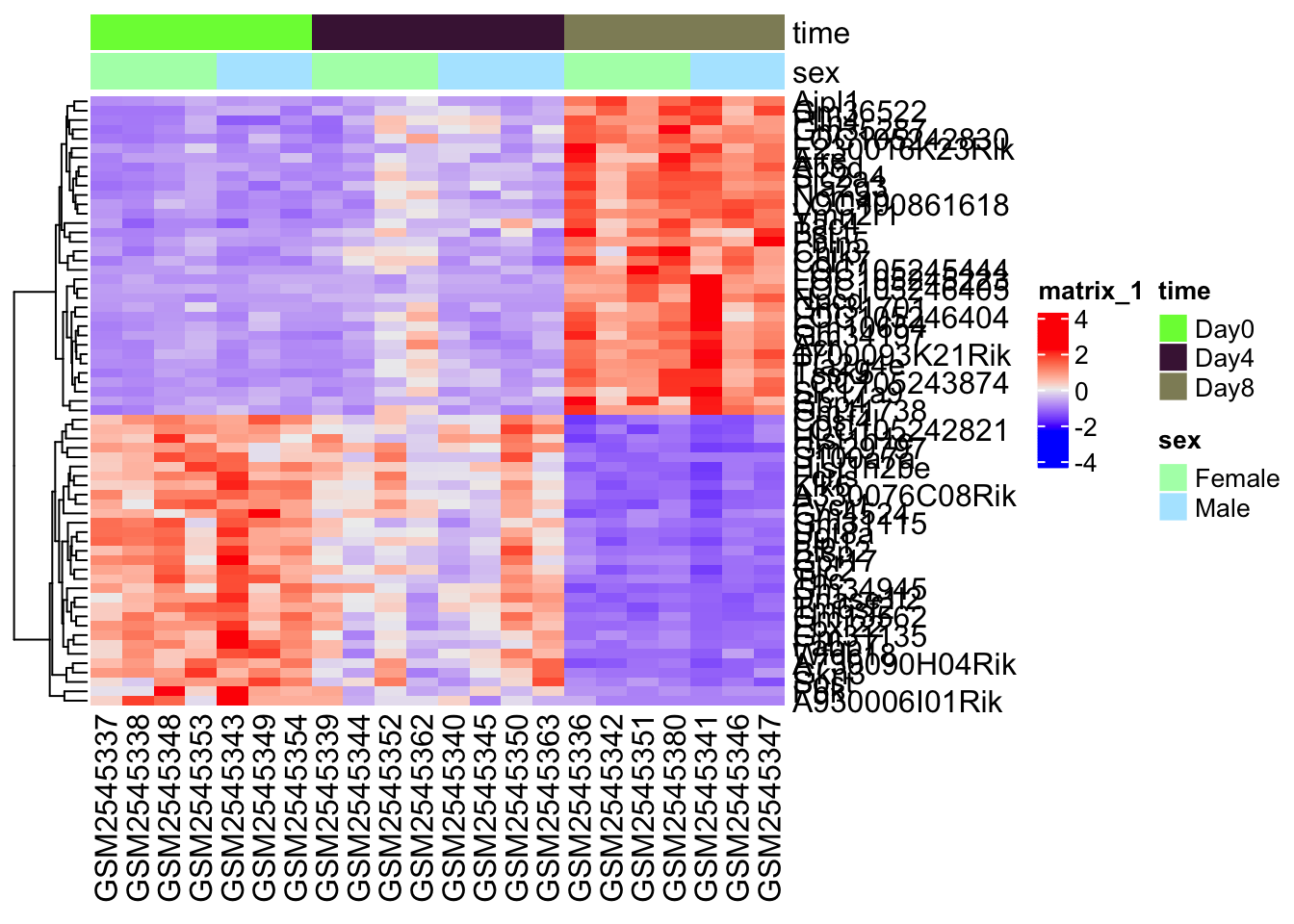

This heatmap is a bit of a mess in terms of the gene annotations, but you can roughly see that there are two large expression patterns, or clusters. This gives us a bit of a clue about possible expression patterns in our data.

We’ll do more about visualizing clusters next week.

6.3 Gene Set Analysis

The basic idea behind gene set analysis is that each gene has a set of annotations attached to them. These may be functional, or may be organized by pathway.

These annotations come from the literature, or functional assays such as protein-protein interactions, or are curated by expert biologists (such as for Reactome).

We first start with our gene set, which has come from our differential expression analysis. This is purely a fictional exercise, but as we can see, we can actually see if our gene set is enriched for annotations.

graph LR
subgraph GeneSet
A[Gene A] 
B[Gene B]
C[Gene C] 
D[Gene D] 
E[Gene E]
F[Gene F]
end
subgraph Terms
G[Cell Cycle]
H[Metabolism]
I[Phosphorylation]
A -- has annotation --> G
B -- has annotation --> G
D -- has annotation --> G
E -- has annotation --> G
F -- has annotation --> G
A -- has annotation --> H
D -- has annotation --> H
A -- has annotation --> I
end
classDef box fill:#DDD
classDef box2 fill:#DFF
class GeneSet box
class Terms box2

We can see that at least 5 out of the 6 genes in our set have the annotation “Cell Cycle”, which seems like it’s over-represented in our Gene Set.

graph LR
subgraph GeneSet
A[Gene A] 
B[Gene B]
C[Gene C] 
D[Gene D] 
E[Gene E]
F[Gene F]
end
subgraph Terms
G[Cell Cycle]
H[Metabolism]
I[Phosphorylation]
end
A -- has annotation --> G
B -- has annotation --> G
D -- has annotation --> G
E -- has annotation --> G
F -- has annotation --> G
classDef box fill:#DDD
classDef box2 fill:#DFF
class GeneSet box
class Terms box2

But what metabolism, which only has two annotations in our gene set? Is that annotation representative of our gene set?

graph LR
subgraph GeneSet
A[Gene A] 
B[Gene B]
C[Gene C] 
D[Gene D] 
E[Gene E]
F[Gene F]
end
subgraph Terms
G[Cell Cycle]
H[Metabolism]
I[Phosphorylation]
end
A -- has annotation --> H
D -- has annotation --> H
classDef box fill:#DDD
classDef box2 fill:#DFF
class GeneSet box
class Terms box2

We need a way to decide which terms are overrepresented, that is occur more than we expected in our analysis. There are statistical approaches to decide this.

In the end, each Term or annotation will have an associated p-value with them. Our alpha cutoff will determing which GeneSets get which annotations.

graph LR
subgraph GeneSet
A[Gene A] 
B[Gene B]
C[Gene C] 
D[Gene D] 
E[Gene E]
F[Gene F]
end
subgraph Terms
G["Cell Cycle<br>p=0.001"]
H["Metabolism<br>p=0.07"]
I["Phosphorylation<br>p=0.1"]
A -- has annotation --> G
B -- has annotation --> G
D -- has annotation --> G
E -- has annotation --> G
F -- has annotation --> G
A -- has annotation --> H
D -- has annotation --> H
A -- has annotation --> I
end
classDef box fill:#DDD
classDef box2 fill:#DFF
classDef green fill:#DFD
class GeneSet box
class Terms box2
class G green

This kind of overrepresentation analysis can be done for any kind of annotation, as long as these annotations are well-curated and we have annotations for a large portion of all genes.

library(SummarizedExperiment)
library(tidySummarizedExperiment)
library(tidyverse)
library(DESeq2)

GSE96870 <- readRDS("data/GSE96870_se.rds")

6.4 Where do these annotations come from?

There are number of annotation packages available for Bioconductor. They are largely organized by organism.

For us, the most important annotation package is org.Mm.eg.db, which contains the mouse genome annotations. There is also org.Hsa.eg.db, which are the Human Genome Annotations.

Gene annotations represent prior knowledge of what is the general shared biological attribute of genes. For example, in a “cell cycle” annotation, all the genes are involved in the cell cycle process. Thus, if DE genes are significantly enriched in the “cell cycle” gene set, which means there are significantly more cell cycle genes differentially expressed than expected, we can conclude that the normal function of cell cycle process may be affected.

As we have mentioned, genes in the gene set share the same “biological attribute” where “the attribute” will be used for making conclusions. The definition of “biological attribute” is very flexible. It can be a biological process such as “cell cycle”. It can also be from a wide range of other definitions, to name a few:

• Locations in the cell, e.g. cell membrane or cell nucleus.
• Positions on chromosomes, e.g. sex chromosomes or the cytogenetic band p13 on chromome 10.
• Target genes of a transcription factor or a microRNA, e.g. all genes that are transcriptionally regulationed by NF-κB.
• Signature genes in a certain tumor type, i.e. genes that are uniquely highly expressed in a tumor type.

We will talk more about annotation sources and databases in a later section.

6.5 How Many Genes have an annotation at random?

In order to do this, we can define a null distribution, or baseline of how many genes have a particular annotation in our gene set.

There are a couple of approaches we can use to determine the statistical significance of an overrepresented annotation. One of the most straightforward is using Fisher’s exact test. What we are comparing are:

• The proportion of genes in our set that have the “cell cycle” annotation (5/6)
• The proportion of genes not in our set that have the “cell cycle” annotation (845/41786)

With a normalizing factor, we arrive at the Fisher’s test statistic, from which a p-value can be derived.

	With Cell Cycle	No cell cycle	Total
In Set	5	1	6
Not in Set	845	40935	41780
Total	850	40936	41786

To do this, we will need to first input our 2 x 2 matrix:

two_matrix = matrix(c(5, 1, 845, 40935), nrow = 2, byrow = TRUE)
two_matrix

     [,1]  [,2]
[1,]    5     1
[2,]  845 40935

Then we can run our Fisher’s test:

test_cell_cycle <- fisher.test(two_matrix, alternative="greater")
test_cell_cycle

    Fisher's Exact Test for Count Data

data:  two_matrix
p-value = 2.031e-08
alternative hypothesis: true odds ratio is greater than 1
95 percent confidence interval:
 34.74055      Inf
sample estimates:
odds ratio 
     243.4 

We can extract the p-value by using the $ operator:

test_cell_cycle$p.value

[1] 2.030933e-08

The interpretation of this is that cell cycle is overrepresented in our small gene set, since it is unlikely that our proportion (5/6) was generated by chance.

In practice, we actually use a faster method for calculating this called the hypergeometric distribution.

You don’t have to do these calculations!

Just a quick note that you don’t have to do these calculations manually. We’ll use the clusterProfiler package to automate this.

We also need to adjust for multiple comparisons, which clusterProfiler does as well.

6.6 Back to Annotations

One of the most common sets of annotations we use are the Gene Ontology annotations. These are divided into 3 different types of annotations:

• Biological Process (BP) - the larger biological processes that gene/protein participates in, such as Cell Cycle
• Cellular Components (CC) - where that gene/protein is localized, such as mitochondria
• Molecular Function (MF) - molecular level activities a gene/protein participates in, such as receptors

When we conduct a Gene Set enrichment analysis, we need to select one or all of these branches.

Gene Ontology annotations are also hierarchical, and have parent annotations, as you can see from the example below:

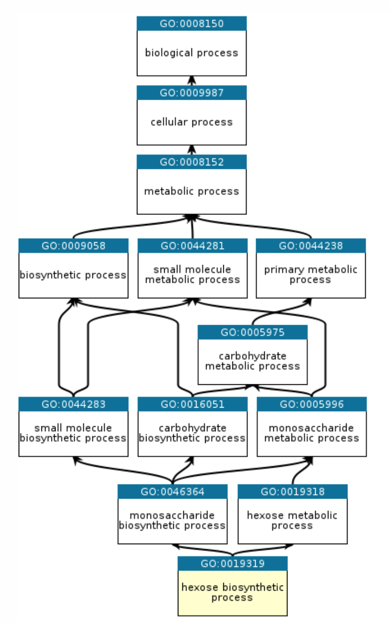
That means that we can actually conduct this analysis at different levels of specificity. For example, we might want to “roll up” more specific annotations (“hexose biosynthetic process”) into more general ones (“carbohydrate synthetic process”). In fact, there are subsets of GO annotations called GO subsets that only cover higher level processes.

6.7 Annotating our Gene Set

We can take our gene set and annotate it with the annotations in the org.Mm.eg.db package:

library(org.Mm.eg.db)

Loading required package: AnnotationDbi

Attaching package: 'AnnotationDbi'

The following object is masked from 'package:dplyr':

    select

keytypes(org.Mm.eg.db)

 [1] "ACCNUM"       "ALIAS"        "ENSEMBL"      "ENSEMBLPROT"  "ENSEMBLTRANS"
 [6] "ENTREZID"     "ENZYME"       "EVIDENCE"     "EVIDENCEALL"  "GENENAME"    
[11] "GENETYPE"     "GO"           "GOALL"        "IPI"          "MGI"         
[16] "ONTOLOGY"     "ONTOLOGYALL"  "PATH"         "PFAM"         "PMID"        
[21] "PROSITE"      "REFSEQ"       "SYMBOL"       "UNIPROT"     

These are all of the various annotations we can utilize. We’ll use them with the clusterProfiler package to conduct our enrichment analysis.

The clusterProfiler package lets us conduct a GO analysis using the org.Mm.es.db, if we use it as an argument.

library(clusterProfiler)

clusterProfiler v4.14.6 Learn more at https://yulab-smu.top/contribution-knowledge-mining/

Please cite:

Guangchuang Yu, Li-Gen Wang, Yanyan Han and Qing-Yu He.
clusterProfiler: an R package for comparing biological themes among
gene clusters. OMICS: A Journal of Integrative Biology. 2012,
16(5):284-287

Attaching package: 'clusterProfiler'

The following object is masked from 'package:AnnotationDbi':

    select

The following object is masked from 'package:purrr':

    simplify

The following object is masked from 'package:IRanges':

    slice

The following object is masked from 'package:S4Vectors':

    rename

The following object is masked from 'package:stats':

    filter

go_results <- enrichGO(
  gene = geneset, 
                     keyType = "SYMBOL",   ## Our geneset is in Gene symbols
                     ont = "ALL",          ## Pick all 3 branches
                     OrgDb = org.Mm.eg.db,
                     pvalueCutoff = 1,
                     qvalueCutoff = 1
)

go_table <- as.data.frame(go_results)

Let’s look at the enrichment results and filter with an adjusted p-value cutoff (p.adjust) of 0.1. The interpretation of the adjusted p-value is that we accept that 10% (0.1) of our findings are potential false discoveries.

go_table |>
  filter(p.adjust < 0.1) |>
  arrange(p.adjust)

In our case, we see that our gene set has genes associated with structural constituent of myelin sheath, regulation of inflammatory response, among other annotations.

Note that these results may be different than the paper’s results due to differences in how we processed the data. Unfortunately, we don’t have the code for this paper so we can completely reproduce our results.

I did attempt to run the enrichKEGG() analysis, but it appears that the data source it queries (KEGG), has changed their API, so I couldn’t get it to work.

6.8 Plotting GO results

The enrichplot package (installed when you install clusterProfiler) can help us visualize our GO results.

library(enrichplot)

enrichplot v1.26.6 Learn more at https://yulab-smu.top/contribution-knowledge-mining/

Please cite:

Guangchuang Yu, Fei Li, Yide Qin, Xiaochen Bo, Yibo Wu and Shengqi
Wang. GOSemSim: an R package for measuring semantic similarity among GO
terms and gene products. Bioinformatics. 2010, 26(7):976-978

enrichplot::dotplot(go_results, showCategory=15)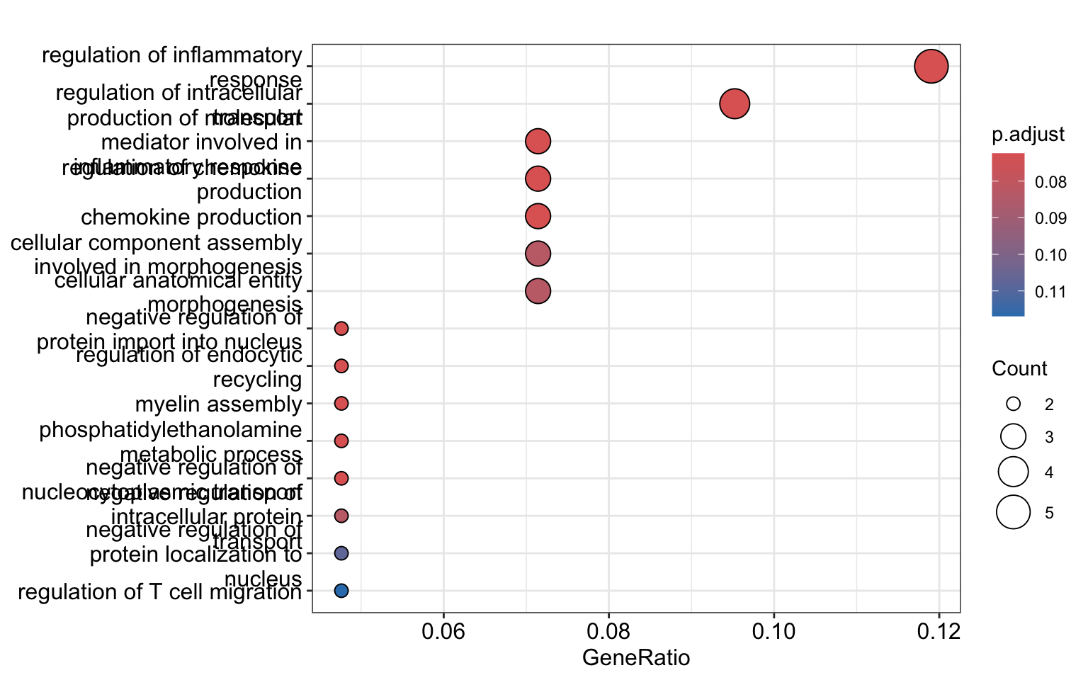

6.9 Translating Gene IDs

There are a number of ways to translate our gene symbols to other identifiers with the bitr() function in clusterProfiler.

entrez_geneset <- 
  bitr(geneset, 
       fromType = "SYMBOL",    ##Our original identifier type
       toType = "ENTREZID",    ##The identifiers we want to translate
       OrgDb = org.Mm.eg.db,   ##The database
       drop = FALSE)           ##Retain those values we don't match

'select()' returned 1:1 mapping between keys and columns

Warning in bitr(geneset, fromType = "SYMBOL", toType = "ENTREZID", OrgDb =
org.Mm.eg.db, : 18.46% of input gene IDs are fail to map...

entrez_geneset

You can see it contains our original gene symbol with the mapped entrez ids.

6.10 Take Home Points

• Once we have filtered our DE candidates, we can treat them as a gene set
• There are annotation packages that let us annotate our GeneSets available in Bioconductor
• clusterProfiler lets us conduct our GO analyses and plot the results.